Auto-Redistrict

2018.05.11:My submission to the Election Law Journal, and the awful horrible very bad reviewers who reviewed it.

Intro

Some time ago, my co-author and I submitted an academic paper to the Election Law Journal. In it we presented two things:

A way to measure gerrymandering that is less counterfactual than other methods, and thus would better stand up to legal arguments.
A method for assessing durability of gerrymandering that can be combined with any measure of gerrymandering.

We were anticipating being “accepted with major revisions”, ‘cause we both know that academic peer review can be brutal. But what we did not expect was that the peer reviewers would be so... incompetent. Not only did they lack a rudimentary understanding of the basic math, but their reading comprehension was so bad that by all appearances they failed to read an entire section of our paper.

To be clear, I do not make these criticisms out of spite, I make them because the evidence supports them. And in what follows I will provide said evidence. I will provide our paper in its entirety, their reviews in their entirety, and I will discuss their reviews point for point. In the end, there will be no room for doubt. Each error a reviewer make is a very basic error, which they repeat multiple times, and which the entire premise of their reviews depend on.

A different way to look at probability

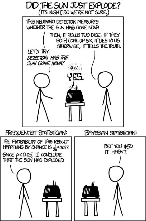
To make this more accessible to more people, allow me to briefly explain the differences between two different ways of working with probabilities: Frequentist vs Bayesian. To put it simply, they both start with Frequentism. Bayesian then builds off of that, much like algebra builds off of arithmetic.

The approach that you are familiar with is the Frequentist approach. For example you estimate the weight of a coin based on the outcome of so many flips, and then from that you can calculate the probability that the next flip will be heads, or the next 10 flips will have 3 heads, etc.

The Bayesian approach takes a step back from that; it is less presumptuous. It says that we cannot know for certain the weight of the coin after so many flips, we can only know that some weights are more likely and others less. The Bayesian approach takes into account all possible weights, without making a definite statement about the weight of the coin, while still using the observations to improve predictions as best as can be done.

While the frequentist approach estimates a single "most likely" weight of the coin, the Bayesian approach calculates an entire spectrum of likelihoods for every possible weight of the coin.

The Bayesian approach is made possible by a key realization discovered by Thomas Bayes, from which the Bayesian approach gets its name:

The probability, after so many observed flips, that a coin has a given weight, is proportional to the probability of observing those flips, if the coin has that weight.

It takes a bit of mental effort to grasp that twist -- that inversion -- no doubt. But from this simple rule one can move from a simple "best guess" approach, to an infinitely more detailed "weighted guesses" approach, as depicted above. This simple reversal is so powerful and versatile, has reverberated to so many fields, that it is often and by many considered the most important mathematical realization known to man.

Opinions about its general importance aside, it's applicability to measures of gerrymandering and quantifying social issues in general cannot be understated. Not only does it provide a more accurate method to analyze any data, social or not, but it provide a clear path to assessing durability; the persistence of an effect over time. For example, in the case of predicting the outcome of the next coin flip, it takes into account that it only has limited data based on a finite number of previous flips, and gives instead of a single probability - such as 50/50 - it gives instead a probability for every probability - such as 30% that it's between 40/60 and 60/40, 10% that it's between 30/70 and 40/60, etc. This kind of data would clearly be more valuable to a court considering the impact of redistricting as compared to changes in voter sentiment, than data acquired by the simpler and less informative Frequentist approach would be.

Additionally, with the Bayesian approach, you can combine all possible weights of the coin, in proportional to their probability, and use that as a "prediction" of what the next flip of the coin will be. This prediction will invariably be more accurate than one made with the Frequentist approach.

So why then does anyone use the Frequentist approach? Well the simple answer is it's easier. But when it comes to the mathematics this means more than you think it does; it's not simply "less work". With the Frequentist approach you can usually do algebra on it to find an exact solution. With the Bayesian approach, usually not. Usually the only way to find a solution is to plug in a bunch of different weights for the coin and see what comes out of each after so many calculations. Now this is trivial today on a computer: you just write a program to do it. But back when these methods were developed they didn't have computers. And thus for practical reasons, everybody used the Frequentist approach on most real-world problems, and that's what was taught.

With that preamble aside, let me finally get into the guts of the peer review. Now mind you, we asked up front that they find peer reviewers knowledgeable in the Bayesian approach. Most mathematicians to this day haven't learned about the Bayesian approach, and we use it a lot in our paper.

After talking with the publisher afterwards, I'm told that one of them was an "expert" in Bayesian analysis. But for the life of me, I can't tell which one is. I certainly hope it is the first, for the second got just about everything about it wrong. And at such a basic conceptual level that I imagine that after my very brief explanation, the average reader can understand their errors.

A link to the full paper

https://github.com/ColinMcAuliffe/UnburyTheLead/raw/master/EmpiricalBayes.pdf

The peer reviews

I recommend this paper not be published in ELJ. The paper suffers conceptual and analytical shortcomings that preclude the authors from delivering on the purpose they have in mind. After explaining what I see as its shortcomings, I conclude with a suggestion for why and how the authors might pursue their argument and analysis with either a different purpose in mind or a different analytical framework.

The authors say, rightly as it pertains to packing gerrymanders, that “to properly assess the harm caused by partisan gerrymandering, courts require mathematical tools for analyzing partisan bias in a redistricting plan” (p. 1). After defining partisan bias as the “discrepancy in seats won by the losing party under a reversal in statewide partisanship” (p. 2), the authors propose a measure of bias called specific symmetry. It refers to “the deviation of the seats votes curve from the symmetry line measured at the statewide popular vote.” To take account of the variability that likely occurs throughout a redistricting cycle the authors put together a Bayesian modelling framework. They apply their model to nationwide U.S. House election 1972-2016 and to Wisconsin Assembly elections after 2010. For both applications they use the election results of the House and Assembly elections.

This is all introduction so far.

Conceptual shortcomings arise from the fact that electoral bias has several sources other than partisan gerrymandering. When looking to “assess the harm caused by partisan gerrymandering,” it is not acceptable to ignore bias arising from these other sources. If we do, we conflate bias-associated harm caused by gerrymandering with bias-associated harm caused by other sources. One of the other sources is residential patterns. While most analyses of gerrymandering seek to distinguish “accidental” districting effects from chosen gerrymanders, perhaps the authors want to argue that the distinction should be ignored by analysts and courts. If they want to make that argument, then they have to present the argument in their text.

The reviewer makes this same claim again later in the review. To save from repetition, it's addressed there and here I say only refer to that section.

Furthermore, if they want to make that argument and to go so far as to say courts should ignore residential patterns as a source, then to publish in ELJ they need to ground their prescription in law and jurisprudence.

This paragraph begins with an “if”; with a hypothetical. That alone should disqualify it, since it’s already a clear acknowledgement that it doesn’t pertain to what was written. And the reviewer is supposed to review what was written, not what hypothetically might be written.

The reviewer then goes on to make a false assertion “to publish in ELJ they need to ground their prescription in law and jurisprudence. “ This is clearly not true. Even if we were to hypothetically write a paper about that - which we did not - such a paper could, for example, be grounded in mathematics, as many such papers published in ELJ have been.

A second source of electoral bias not directly attributable to chosen gerrymanders arises from the competition within districts, especially as it relates to incumbency. The incumbency-bias connection was Bob Erikson’s point back in 1972, and it was Gelman and King’s point in the early/mid 1990s. The role of incumbency is clearly evident in the authors’ Figure 7. If it is not evident to the authors, all they need to do is compared their Figure 7 histograms to similarly constructed distributions for the presidential vote by districts.

This isn’t even a critique of the paper - it’s just a commentary; an aside. If the reviewer wants to write a paper about incumbency effects, we’re not stopping them. (It’s not particularly novel, though.) We didn’t bother with this because our paper is already complex enough as it is. This is the norm - many if not most published papers don’t account for incumbency. For example, papers on the efficiency gap, published in ELJ, don’t account for incumbency. One wonders if the reviewer was reviewing those papers, would they have the same commentary? Is it the reviewers opinion that none of those papers should have gotten published, due to their not analyzing incumbency? This would drastically reduce the numbers of papers published. And I don’t think that would be a positive contribution for academia.

It is also important to point out that readers are left to wonder what is innovative about the conceptual innovation the authors appear to have in mind.

From the abstract:

“Additionally, we propose a new measure of gerrymandering called the specific asymmetry which we believe will stand up better to judicial and technical tests than any other measure proposed thus far. The specific asymmetry does not rely on proportionality of seats and votes, is applicable to any level of statewide partisanship, does not require national results as a baseline, and measures bias at the popular vote that actually occurred as opposed to some other hypothetical popular vote. All other available metrics fall short in at least one of these aspects, which leaves them vulnerable to criticism and manipulation by those seeking to gerrymander or to defend an existing gerrymander.”

From Section 2:

“Measuring Bias with the Specific Asymmetry Measuring partisan bias accurately presents several challenges from a mathematical and legal perspective. Redistricting will always be an artificial process, and therefore we must establish what characteristics of a redistricting plan can be regarded as normative before attempting to measure deviations from the normative standard. We propose the following definition: a fair redistricting plan is one that, on average, will not be biased in favor of either of the two major parties. With this definition in mind, we turn our attention to several challenges in devising a metric for bias. First, single winner elections tend not to produce proportional outcomes [1], and we therefore can not use proportionality or the lack thereof as a measure of bias. Bias should therefore be a measure of symmetry, which permits disproportionate outcomes but requires that any advantage that might arise from the disproportionate nature of the single winner election system be equally available to either party. In other words, we say that the result is unbiased if and only if any advantage gained by a party, above what is proportional, is a consequence of the disproportionate nature of the single winner election system, and not an additional advantage piled on top of that.

A few measures of bias that follow this definition exist in the literature, such a Grofman and King, and the mean median difference [7, 2, 3]. However, these measures of bias tend to apply only to states which are close to 50-50 partisanship. For more partisan states, these measures become more difficult to interpret except as the bias which could have occurred had the partisanship in the state in question been closer to even. Another approach is to consider the bias at levels of partisanship by using the geomet the structural disadvantage to one party increases due to a more aggressive gerrymander, the specific asymmetry increases as well. The metric can be calculated deterministically from the results of a single election, and when combined with the sampling method in section 3, a quantity representing the distribution of likely asymmetries analogous to equation 1 can be computed. Sampling the specific asymmetry to compute likely asymmetries is preferable to using the integral in equation 1, since the specific asymmetry has units of seats.

…

There are several other advantages to using this metric, which we summarize below.

…

• It works for states with partisanship far from 50/50 - By sampling the asymmetry at the actual vote counts rather than e.g. 50/50, this metric maintains full relevance even for the most extremely partisan states.

Any “reader” who is “left to wonder” this clearly did not *read* either the abstract, or section 2 of the paper. Apparently, the reviewer is one such (non-)reader.

Now the following couple of paragraphs, which constitute most of this review, are a bit tangled and so a bit difficult to unpack. Fortunately they are almost exclusively about one section of the paper, which the reviewer is clearly very very confused about.

They evaluate bias (asymmetry in their hypothetical vote-to-seat translation) at the vote percentage level in the system-wide vote and imply this is preferred to what has been done previously. While it is different from the Gelman-King and Grofman-King evaluation around the 50 percent mark, the authors offer no explanation for why evaluating bias at a given particular vote percentage is more valuable than knowing about bias at and around the 50 percent mark. We do know, on the other hand, a focus around 50 percent is justified on the basis of a concern for majoritarianism. What is the value of knowing the amount of bias in a state such as Utah where one compares seats won when Republicans win about 60 percent of the vote, as they typically do in Utah since 1980, to what might have happened were Democrats to have won 60 percent of the vote?

From the abstract:

From Section 2:

…

There are several other advantages to using this metric, which we summarize below.

…

From the standpoint of appealing to courts, which the authors say they have in mind and which submission to ELJ underscores they must have in mind, their Beta distribution grounded model builds on assumptions of hypothetical states of affairs that the Justice Kennedy spoke of when he favorably reviewed but ultimately rejected the amicus-presented model discussed in Grofman-King.

This is totally and completely false and shows that the reviewer doesn't even know what a Beta distribution represents, nonetheless what Justice Kennedy meant. Justice kennedy was saying that measuring at a hypothetical 50-50 vote is a hypothetical state of affairs. Our proposed measure avoids this hypothetical by measuring at the actual popular vote instead of a hypothetical 50-50 vote, which is what Justice Kennedy expressed dismay about.

Furthermore it is simply not possible for Kennedy to be referring to the Beta distribution when critiquing Grofman-King, because Grofman-King DOES NOT USE the Beta distribution. Anywhere.

One could maybe imagine a situation where Kennedy mistakenly thought they did, but this would imply not only that Kennedy was very confused by his own vivid imagination, but also that, in addition to being a legal scholar, he was also knowledgeable in a field of mathematics that is esoteric to even many people with a degree in mathematics. A pair of situations that, while alternately flattering and offensive, are extremely unlikely, each taken alone, not to mention in combination.

Regarding the reveiwer’s lack of understanding of Beta distributions, consider the reviewers phrase, and I quote: “Beta distribution grounded model builds on assumptions”. Far from being built on assumptions, a Beta distribution dismantles assumptions. It is a probability distribution on the values of the parameters of yet another probability distribution. Where as the more common frequentist approach estimates a single value for the parameters of a distribution based on the method of moments, Bayesian methods take a step back from that and instead calculate the probability of every potential value for every parameter of a distribution, by using Bayes’ rule. In short, Bayesian analysis very explicitly makes fewer assumptions, resulting in posterior distributions with higher variance. This more accurately and appropriately represents both the amount of uncertainty, and where it is.

This is Bayesian probability 101.

Then, making things even more hypothetical, when the authors apply their model they add data-related assumptions. For both their U.S. House and Wisconsin Assembly analyses, they substitute average or presidential election results for uncontested elections.

As discussed in many sources that we cite, the process of imputing is STANDARD OPERATING PROCEDURE. And more importantly, the two alternatives: throwing out those elections altogether, or treating those elections as if they were contested (by including them un-imputed) gives results that are less accurate, and amounts to lying. In the first case you are saying that the demographics of the state are reflected by only that of contested elections, which is false. In the second case, you are saying elections were contested that were not.

So if the reviewer's complaint is that when confronted with the two alternatives: lying and using a flawed methodology, and lying and using a flawed methodology, we chose instead a third: using the accepted academic practice and imputing, then we stand guilty as charged.

And for the Wisconsin Assembly analysis they “cross aggregate” (p. 12) the 2006-10 election results to the post-2010 districts (p. 12). This apparently involves the heroic assumption that votes in Assembly districts cast when two particular candidates competed can be cross-aggregated to a new set of districts when and where different candidates compete.

Nope. This is a statistical estimate based on demographics. And properly conditioned on Bayesian hyper-priors, which are in turn empirically fitted, which are then in turn regularized to account for uncertainty implicit in the fact that we are trying to predict the NEXT data point, as opposed to previous ones.

All of which I might add, is STANDARD OPERATING PROCEDURE, which apparently the reviewer knows absolutely nothing about.

The authors clearly have put a good deal of thought and effort into this paper. If they pursue it, I suggest they switch their focus in either of two ways. (1) They could keep much of what they are doing and change the focus from gerrymandering to electoral bias. What is presented here is a model and set of analyses on bias from various sources, not just gerrymandering. If they make that switch they will still need to explain the value of the concept of specific asymmetry—bias at the level of the system-wide vote percentage.

We did.

(2) If they want to stick with gerrymandering as their conceptual focal point, they could keep the legislative elections as something like an afterthought to be checked for bias but rely principally on statewide elections to detect gerrymandering bias.

This suggestion is beyond the appropriate scope of a review. If you want to write a paper about that, go ahead. The authors cannot be expected to anticipate ad-hoc analytic inventions of the reviewers.

Doing so removes the large influence of incumbency.

Again, the reviewer is invited to write a paper about this.

It would leave them with the issue of residential patterns to deal with,

We did - they are moot because they are easily counteracted.

and they would again have to deal with explaining the value of the concept of specific symmetry.

Again, we did.

Reviewer 2 review:

Reviewer: 2

Comments to the Author

This paper presents a new measure and method of evaluating gerrymandering. While the topic is obviously important, the proposed methodology has a number of problems.

Most importantly, to evaluate gerrymandering, one cannot just look at election outcomes. Instead, researchers must examine the election outcomes within the context of geographical and other features (e.g., distribution of different types of voters) of each state.

ALL proposed measures of gerrymandering would fail this test. And yet, they were published.

The authors ignore these important complexities

and propose a method that assumes an election outcome for each district is independently, and identically distributed.

False. We

explicitly identify and talk about weaknesses with the i.i.d. assumption and
avoid having to make it by:

using a Bayesian Empirical method,
using Monte-Carlo Integration, and

explicitly do NOT make the i.i.d. assumption by subtracting the shared variance via the statewide popular vote. That is, we account for correlations among all districts by estimating a single parameter weighted by vote count. This parameter represents statewide (or more generally election-wide) covariance.

The alternative, computing a full matrix of correlations, would violate basic rules of Model Selection. Particularly, it would be incorrect because there are not sufficient samples to support that many extracted parameters. It would be over-fitting.

I do not think that such methods can yield valid inference about gerrymandering.

Well then your beef is not with our paper, but with others that have been published in ELJ. And pretty much all of them, at that, as most published papers on quantitatively measuring gerrymandering are analytic and assume i.i.d., as we discuss in the very intro to our paper. Presumably had you been the reviewer for them, they would have all gotten rejected, leaving academia completely void of papers on quantitatively measuring gerrymandering, except for, ironically, this paper, which does NOT assume i.i.d., uses a Bayesian Empirical method, and uses Monte-Carlo Integration to eliminate the need for i.i.d. assumptions.

** specific comments **

1. The authors review the existing methods, but they do not appear to be aware of the recent work based on Markov chain Monte Carlo.

I'm sorry we didn't review your favorite method. I didn't get the memo that that's what we were supposed to be doing.

Unlike the Monte Carlo methods of Chen and Wang, these methods are designed to obtain a representative sample of redistricting plans from a target population.

Wait, how is that unlike the methods of Chen and Wang? Are Chen and Wang’s methods not designed to obtain a representative sample of redistricting plans from a target population? I’m pretty sure in simulating hundreds of redistricting plans for a target population, they were trying to obtain a representative sample. Also, why are we discussing a different paper?

In contrast, the methods proposed by Chen and Wang do not possess such a theoretical property and can yield a highly biased sample.

I don't see anywhere in the paper where we claim that Chen's samples are unbiased or where we depend on such an assumption.

Because there isn't any.

See the works by Imai and Mattingly and their collaborators.

Wait, are you rejecting our paper on the basis of a perceived flaw in somebody else's paper (which, btw, was NOT rejected by this very journal)?

2. I do not see the advantage of the 'specific asymmetry.' As the authors recognize, the counterfactual considered here seems too far from the observed outcome.

I think the reviewer is swapping Grofman-King asymmetry with specific asymmetry. Whereas they measure at 50-50, which is often quite far from the observed outcome, we measure exactly at the observed outcome. That’s kind of the whole idea. In this case it is clearly Grofman-King that is counterfactual.

Or is the reviewer thinking that by comparing the actual outcome with the reversal (reflection), we are saying this might be perceived as being counterfactual. If so, the author should take a closer look at Grofman King asymmetry and see that it does the same thing. So if the reviewer considers this a reason for specific asymmetry being inferior to Grofman King asymmetry - which in this interpretation they do - then it follows that for this same reason, Grofman King asymmetry is inferior to Grofman King asymmetry.

While the reviewers comment is ambiguous, in either interpretation, he is clearly very confused, and very wrong.

From the abstract:

From Section 2:

…

There are several other advantages to using this metric, which we summarize below.

…

Pretty frickin’ clear.

Why is this better than the usual measure of partisan symmetry?

We've explained that thoroughly in the paper. That's kind of the the entire second section. Also part of the abstract. And the introduction. Also there are multiple bulleted lists. Which one of them did you not read? Oh, that’s right, you’d have to have not read ANY OF THEM!

From the abstract:

From Section 2:

…

There are several other advantages to using this metric, which we summarize below.

…

3. The assumptions of the proposed methodology need to be clearly stated, and the model needs to be more formally presented. As far as I can tell, the author assumes that each election is iid according to the Beta distribution.

This makes no sense. The Beta distribution is a prior, but the reviewer speaks of it as if it is a posterior. That is, it estimates probabilities for parameters of a distribution, but the reviewer treats it as if it assumes certain parameters on a distribution, and then defines a distribution of outcomes. Confusing a prior with a posterior is a fatal flaw in Bayesian analysis that shows a complete lack of understanding of the basic principles of Bayesian methods.

Using a prior that is conditioned on multiple elections assumes exactly the opposite of i.i.d.: it assumes strong dependance.

Is this an appropriate assumption? It seems too simplistic to me. Surely, there is dependence across time periods and across districts within each time period.

Surely there is. That’s why we used a Beta Prior. By using empirical data to estimate a Beta prior on all elections for a set of districts, we are implicitly assuming dependence.

This would be obvious to a reviewer if they knew anything at all about Bayesian empirical methods, or priors for that matter, or Beta distributions.

We are using Beta priors precisely to model dependence within a time period.

He said across though - you can't model across time periods because the districts are different. Unless you deaggregate to a higher resolution and then re-aggregate to the different districts. A method that reviewer 1 asserts is unjustified. Why does reviewer 1 mention that? Because that's exactly what we do in section 4!

Reviewer 1 doesn't appear to recognize that districts change shape between redistricting cycles, a rather trivial and obvious consideration.

Furthermore, he claims that we do not do exactly what we dedicated an entire section to doing, which, mind you, nobody else has ever done.

Earlier in the paper, the authors criticize (rightly) the independence assumption of Wang's method.

So... then.... maybe... we're not assuming iid?

It's also unclear how the estimation uncertainty is accounted for

This is a Bayesian analysis. There is no “estimation uncertainty” because it is not a point estimate. It gives you an entire probability distribution as a result. (called the “posterior predictive distribution”) You want a point estimate of estimation uncertainty? Pick a function, integrate, done. Some popular choices are the second statistical moment, or confidence intervals at 10 and 90. We calculate a couple such point estimates in section 3.

Or are you talking about the prior? Because we used naive Bayes. If the meaning of “naive Bayes” is “unclear” to you, then I suggest you look it up. And look up “posterior predictive distribution” while you’re at it.

Either way, the reviewer clearly doesn't understand the fundamentals of Bayesian analysis.

and how the "shrinkage variance" is chosen.

Do you not know how to read? We put the formula in the paper, surrounded with a very clear explanation. In the subsection titled -- get this -- “Parameter Estimation”!

We use standard unbiased estimator - +1 in the denominator, and double checked that by making sure that in the single sample case it works out.

How could we possibly be any more clear?!

4. The model's advantages are described.

What, did you not earlier say that we never described the model’s advantages?!? (“I do not see the advantage of the 'specific asymmetry.' “) Which one is it? (Hint: it’s this one; they ARE described.)

Again, the simplifying assumptions are problematic here. For example, without modeling time trend, how can one assess "durability"?

We explain that in the paper. Using a Bayesian Empirical Method. We literally dedicated an entire section to it. How much more do you want? Two sections?!?

Also, the Monte Carlo method needs to be formally described.

Look it up in wikipedia? https://en.wikipedia.org/wiki/Monte_Carlo_integration

It’s not “a Monte Carlo method”, it’s “Monte Carlo Integration”, a very rigorously defined algorithm. I don’t think we made any typos with that one. Anticipating the confusion, I was careful to always say “integration”.

5. The authors impute the mean value for uncontested districts without justification.

We impute with plenty of justification, as we explain and cite. And has been explained in many papers before (such as the ones that we cite).

Additionally, we make it clear that we invite others to explore other methods of imputation. As do the papers we cite.

Also, these values are treated as if they are observed and the uncertainty about this imputation procedure is not accounted for.

We cover imputation and cite various resources for you to learn more about it, and clearly invite other methods of imputation.

The usual practice is to treat them as observed values. I mean, you could write a paper about how to expand a model that, via Bayesian method, uses imputation probability distributions, and defers marginalization until integration of the posterior predictive. But that would be a long paper, and for a rather technical audience. (Indeed, that was probably just a garble of words to most readers.) It is far from the norm to use such a detailed model in a simple introduction to a measure, or any paper on measuring partisan bias, for that matter. To confirm this, you can check the numerous papers we cited. None of them do what you describe. We felt our paper was already complicated enough to add yet another topic for people to take in. Clearly, other authors shared this feeling when they wrote their papers, as did the reviewers of those papers, who accepted them for publication.

And clearly, we were right. As the numerous confusions and just lack of actually reading by the reviewers bears testament to.

Closing thoughts

Finally I have something to say about the process that I found myself going through to write all these responses. It took a lot of reading over, and a lot of time and emotional distance, and a few iterations.

This is all expected. Deserved, for the reviewers volunteered their time. But what was not expected was what, in retrospect, was the largest factor that led to so many iterations and so much time: in a word, disbelief.

Disbelief that they could pretend with so much decorum that they know so much about what they are talking about, when it is so obvious to anyone who actually does know, that they know next to nothing about what they're talking about, and pretty much everything they think they know, is just wrong. Disbelief at simultaneously the depths of pretension, and the depths of incompetence.

I might expect this from presidents, but not from scholars. And certainly not two out of two.

It is never a happy experience to write about such a thing, and respect for the feelings of others makes you make every effort to give them the benefit of the doubt. But at long last, every benefit was betrayed, every doubt, confirmed.

In the end, there was no plausible interpretation remaining -- not even remotely -- that wasn’t just downright --- gross. If this was a house on fire, it would be ashes, with not a single support left standing.

As I read it more carefully, more slowly, and with more distance, it only grew worse.

My co-author said we just submit to other journals. I've seen the quality of reviews from two separate people, and they are both 0 for - well I don't really care to count and there's really no point. Just zero. If this is any indication of future reviews, then a “passing review” would be just as arbitrary and nonsensical as a falling one, and I cannot in intellectual good conscience call that a win.

More to the point I cannot abide by a process whose practical outcome is no different than a lottery. I can not submit my intellectual compositions to such arbitrary nonsense. It denigrates them, it insults them. Nor can I sit idly by while others works are so insulted.

You might as well just farm it out to entirely random people on the internet through something like Yahoo answers. At least that way you'll likely get some people who know what they're talking about, even if most of then do not. And if actual paper writers just submit to journal after journal until they get a hit, one might as well just simplify the process and use the law of large numbers up front.

In short, if this is peer review, I’d rather self-publish. It'd be more credible.

Bayesian methods are THE correct way to analyze gerrymandering.

If I would like to leave the reader with any thought - besides my frustration - it is this: the Bayesian approach to probability is fundamentally superior to the Frequentist approach, and when considering quantitative social problems, such as voting, it is just quite simply a more accurate and detailed way to analyze raw data. And if a judge of any court has probability - related questions, I believe a short introduction to Bayesian methods like I gave in the intro is appropriate.